Nucleus Instance Segmentation¶

Click to open in: [GitHub][Colab]

About this demo¶

Each WSI can contain up to million nuclei of various types, which can be further analysed systematically and used for predicting clinical outcomes. In order to use nuclear features for downstream analysis within computational pathology, nucleus segmentation and classification must be carried out as an initial step. However, this remains a challenge because nuclei display a high level of heterogeneity and there is significant inter- and intra-instance variability in the shape, size and chromatin pattern between and within different cell types, disease types or even from one region to another within a single tissue sample. Tumour nuclei, in particular, tend to be present in clusters, which gives rise to many overlapping instances, providing a further challenge for automated segmentation, due to the difficulty of separating neighbouring instances.

Image courtesy of Graham, Simon, et al. “Hover-net: Simultaneous segmentation and classification of nuclei in multi-tissue histology images.” Medical Image Analysis 58 (2019): 101563.

In this example, we will demonstrate how you can use the TIAToolbox implementation of HoVer-Net to tackle these challenges and solve the problem of nuclei instance segmentation and classification within histology images. HoVer-Net is a deep learning approach based on horizontal and vertical distances (and hence the name HoVer-Net) of nuclear pixels to the centre of mass of the corresponding nucleus. These distances are used to separate clustered nuclei. For each segmented instance, the nucleus type is subsequently determined via a dedicated up-sampling branch.

In this example notebook, we are not going to explain how HoVer-Net works (for more information we refer you to the HoVer-Net paper), but we will show how easily you can use the sophisticated HoVer-Net model, which is incorporated in TIATtoolbox, to do automatic segmentation and classification of nucleus instances. Mostly, we will be working with the NucleusInstanceSegmentor which by default uses one of the pretrained HoVerNet models. We will also cover the visualisation tool embedded in TIAToolbox for overlaying the instance segmentation results on the input image.

Note: NucleusInstanceSegmentor is a deprecated wrapper around MultiTaskSegmentor and will be removed in a future release.

Downloading the required files¶

We download, over the internet, image files used for the purpose of this notebook. In particular, we download a histology tile and a whole slide image of cancerous breast tissue samples to show how the nucleus instance segmentation model works.

In Colab, if you click the files icon (see below) in the vertical toolbar on the left hand side then you can see all the files that the code in this notebook can access. The data will appear here when it is downloaded.

# These files are used for the experiments
img_file_name = global_save_dir / "sample_tile.png"
wsi_file_name = global_save_dir / "sample_wsi.svs"


logger.info("Download has started. Please wait...")

# Downloading sample image tile
download_data(
    "https://huggingface.co/datasets/TIACentre/TIAToolBox_Remote_Samples/resolve/main/sample_imgs/breast_tissue_crop.png",
    img_file_name,
)

# Downloading sample whole-slide image
download_data(
    "https://huggingface.co/datasets/TIACentre/TIAToolBox_Remote_Samples/resolve/main/sample_wsis/wsi4_12k_12k.svs",
    wsi_file_name,
)

logger.info("Download is complete.")

Nucleus instance segmentation and classification using TIAToolbox’s pretrained HoVer-Net model¶

In this section, we will investigate the use of the HoVer-Net model that has been already trained on the PanNuke dataset and incorporated in the TIAToolbox. The model we demonstrate can segment out nucleus instances in the image and assign one of the following 6 classes to them:

Background
Neoplastic Epithelial
Non-Neoplastic Epithelial
Inflammatory
Connective
Dead

Inference on tiles¶

Similarly to the semantic segmentation functionality of the TIAToolbox, the instance segmentation module works on image patches, tiles and structured WSIs. First, we need to create an instance of the NucleusInstanceSegmentor class which controls the whole process of the nucleus instance segmentation task and then use it to do prediction on the input image(s):

# Tile prediction
inst_segmentor = NucleusInstanceSegmentor(
    model="hovernet_fast-pannuke",
    num_workers=0,  # Change to multiprocessing.cpu_count() to use all available cores
    batch_size=4,
    device=device,
)

output = inst_segmentor.run(
    images=[img_file_name],
    save_dir=global_save_dir / "sample_tile_results/",
    patch_mode=False,
    input_resolutions=[{"units": "baseline", "resolution": 1.0}],
    auto_get_mask=False,
)

There we go! With only two lines of code, thousands of images can be processed automatically. There are various parameters associated with NucleusInstanceSegmentor. We explain these as we meet them while proceeding through the notebook. Here we explain only the ones mentioned above:

model: specifies the name of the pretrained model included in the TIAToolbox (case sensitive) or a model instance. We are expanding our library of models pretrained on various (instance) segmentation tasks. You can find a complete list of currently available pretrained models here. In this example, we use the "hovernet_fast-pannuke" pretrained model, which is a HoVer-Net model trained on the PanNuke dataset. Another option for HoVer-Net is hovernet_original-kumar which is the original version of the HoVer-Net model trained on a dataset by Kumar et al..
num_workers: controls the number of CPU workers used for data loading and post-processing.
batch_size: controls the batch size, or the number of input instances to the network in each iteration. If you use a GPU, be careful not to set the batch_size larger than the GPU memory limit would allow.
device: specify appropriate device e.g., "cuda", "cpu" etc.

After the inst_segmentor has been instantiated as the instance segmentation engine with our desired pretrained model, we call the run method to do inference on a list of input images (or WSIs). The run function automatically processes all the images in the input list and returns the results. The process usually comprises patch extraction (because the whole tile or WSI won’t fit into limited GPU memory), preprocessing, model inference, post-processing and prediction assembly. Here are some important parameters for the run method:

images: list of inputs to be processed. Items in the list should be paths to the inputs, WSIReader objects, or NumPy arrays.
patch_mode: set to True for patches (inputs must match the model’s expected patch size) and False for WSIs/tiles where patch extraction is required.
save_dir: path to the main folder in which prediction results are stored (required only if output_type is "zarr" or "annotationstore").
input_resolutions: read resolution for input extraction. “baseline” with 1.0 means use full‑resolution (level 0) coordinates when extracting patches/tiles.
auto_get_mask: when patch_mode=False, automatically generate a tissue mask if masks is not provided. Here it is set to False to process the whole tile without masking.

# Load the output tile predictions from disk
# The returned dictionary `output` maps each tile path to
# its corresponding `.zarr` file.
# We load the output tile predictions into memory as below.

store_path = output[img_file_name]
tile_output = zarr.open(store_path, mode="r")
logger.info(f"Output keys: {list(tile_output.keys())}")

|2026-02-20|09:28:12.011| [INFO] Output keys: ['box', 'centroid', 'contours', 'coordinates', 'prob', 'type']

The tile_output Zarr group contains one array per field (e.g., box, centroid, contours, prob, type). Each array is indexed by instance, so the i‑th entry across arrays describes the same nucleus.

tile_output = {
  box:      [ [x_min, y_min, x_max, y_max], ... ],
  centroid: [ [x, y], ... ],
  contours: [ [ [x, y], [x, y], ... ], ... ],
  prob:     [ p, ... ],
  type:     [ t, ... ],
}

Below, we convert the output Zarr group into a per-instance dictionary (tile_preds) that is convenient for visualization.

# Convert the output to the legacy per-instance dict expected by
# overlay_prediction_contours().
tile_preds = {}
for inst_id, (box, centroid, contour, prob, type_id) in enumerate(
    zip(
        tile_output["box"],
        tile_output["centroid"],
        tile_output["contours"],
        tile_output["prob"],
        tile_output["type"],
        strict=False,
    ),
    start=1,
):
    tile_preds[inst_id] = {
        "box": box,
        "centroid": centroid,
        "contour": contour,
        "prob": float(prob) if prob is not None else None,
        "type": int(type_id) if type_id is not None else None,
    }

logger.info(f"Number of detected nuclei: {len(tile_preds)}")

# Extracting the nucleus IDs and select the first one
nuc_id_list = list(tile_preds.keys())
selected_nuc_id = nuc_id_list[0]
logger.info(f"Nucleus prediction structure for nucleus ID: {selected_nuc_id}")
sample_nuc = tile_preds[selected_nuc_id]
sample_nuc_keys = list(sample_nuc)
logger.info(
    "Keys in the output dictionary: [%s, %s, %s, %s, %s]",
    sample_nuc_keys[0],
    sample_nuc_keys[1],
    sample_nuc_keys[2],
    sample_nuc_keys[3],
    sample_nuc_keys[4],
)
logger.info(
    "Bounding box: (%d, %d, %d, %d)",
    sample_nuc["box"][0],
    sample_nuc["box"][1],
    sample_nuc["box"][2],
    sample_nuc["box"][3],
)
logger.info(
    "Centroid: (%d, %d)",
    sample_nuc["centroid"][0],
    sample_nuc["centroid"][1],
)

|2026-02-20|09:28:21.467| [INFO] Number of detected nuclei: 484
|2026-02-20|09:28:21.468| [INFO] Nucleus prediction structure for nucleus ID: 1
|2026-02-20|09:28:21.468| [INFO] Keys in the output dictionary: [box, centroid, contour, prob, type]
|2026-02-20|09:28:21.468| [INFO] Bounding box: (46, 0, 65, 6)
|2026-02-20|09:28:21.469| [INFO] Centroid: (54, 1)

We can visualize the predicted contours of the nuclei overlaid on the original image tile as below:

# Reading the original image
tile_img = imread(img_file_name)

# defining the coloring dictionary:
# A dictionary that specifies a color to each class {type_id : (type_name, colour)}
color_dict = {
    0: ("background", (255, 165, 0)),
    1: ("neoplastic epithelial", (255, 0, 0)),
    2: ("Inflammatory", (255, 255, 0)),
    3: ("Connective", (0, 255, 0)),
    4: ("Dead", (0, 0, 0)),
    5: ("non-neoplastic epithelial", (0, 0, 255)),
}

# Create the overlay image
overlaid_predictions = overlay_prediction_contours(
    canvas=tile_img,
    inst_dict=tile_preds,
    draw_dot=False,
    type_colours=color_dict,
    line_thickness=2,
)

# showing processed results alongside the original images
fig = plt.figure()
ax1 = plt.subplot(1, 2, 1), plt.imshow(tile_img), plt.axis("off")
ax2 = plt.subplot(1, 2, 2), plt.imshow(overlaid_predictions), plt.axis("off")

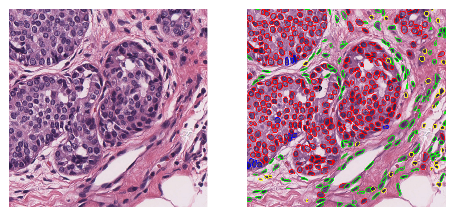
../../_images/48bccfbb14fe3955ea2a517e5413605af6c635e9ced7861382a4040505fe496e.png

As you can see, overlay_prediction_contours beautifully generates an image that has the instance segmentation classification overlaid. Here are the explanations regarding this function’s arguments:

canvas: the image on which we would like to overlay the predictions. This is the same image as the input to the run method, loaded as a NumPy array.
inst_dict: predicted instance dictionary. Here we use tile_preds, which is converted from the tile_output dictionary into a per-instance format expected by the visualization utility.
draw_dot: specifies whether to show detected nucleus centroids on the overlap map. Default is False.
type_colours: a dictionary containing the name and colour information for each class in the prediction. The HoVer-Net model in this example has 6 nucleus classes which are defined above.
line_thickness: specifies the thickness of contour lines.

Inference on WSIs¶

The next step is to use TIAToolbox’s embedded model for nucleus instance segmentation on a whole slide image. The process is quite similar to what we have done for tiles. We will just introduce some important parameters that configure the instance segmentor for WSI inference.

Please note that this part may take too long to process, depending on the system you are using (GPU enabled/disabled) and how large the input WSI is.

# Instantiate the nucleus instance segmentor
inst_segmentor = NucleusInstanceSegmentor(
    model="hovernet_fast-pannuke",
    num_workers=multiprocessing.cpu_count(),
    batch_size=16,
    device=device,
    verbose=True,
)

# WSI prediction
# if device="cpu", this part will take quite long to process.
wsi_output = inst_segmentor.run(
    images=[wsi_file_name],
    masks=None,
    patch_mode=False,
    save_dir=global_save_dir / "sample_wsi_results/",
    output_type="zarr",
    auto_get_mask=False,
)

Note some important parameters here:

Passing auto_get_mask=False to run. If True and if no masks input is provided, the toolbox will extract tissue masks from WSIs.
Setting patch_mode=False in the arguments to run tells the program that the inputs are not in patch format.
masks=None: the masks argument to run is handled in the same way as the images argument. It is a list of paths to the desired image masks. Patches from images are only processed if they are within a masked area of their corresponding masks. If not provided (masks=None), then a tissue mask is generated for whole-slide images or, for image tiles, the entire image is processed. In this example, we leave auto_get_mask=False because we are using a WSI that contains only tissue region (there is no background region) and therefore there is no need for tissue mask extraction.

The above code cell might take a while to process, especially if device="cpu". The processing time mostly depends on the size of the input WSI. The output, wsi_output, of run contains a dictionary mapping each input WSI to its output .zarr file saved on disk. We open that Zarr group and convert it into a per-instance dictionary for inspection and visualization.

wsi_zarr_path = next(iter(wsi_output.values()))
wsi_zarr = zarr.open(str(wsi_zarr_path), mode="r")

# Convert WSI output to the legacy per-instance dict expected by
# overlay_prediction_contours.
wsi_pred = {}
for inst_id, (box, centroid, contour, prob, type_id) in enumerate(
    zip(
        wsi_zarr["box"][:],
        wsi_zarr["centroid"][:],
        wsi_zarr["contours"][:],
        wsi_zarr["prob"][:],
        wsi_zarr["type"][:],
        strict=False,
    ),
    start=1,
):
    wsi_pred[inst_id] = {
        "box": box,
        "centroid": centroid,
        "contour": contour,
        "prob": float(prob) if prob is not None else None,
        "type": int(type_id) if type_id is not None else None,
    }

logger.info("Number of detected nuclei: %d", len(wsi_pred))

# Extracting the nucleus IDs and select a random nucleus
rng = np.random.default_rng()
nuc_id_list = list(wsi_pred.keys())
selected_nuc_id = nuc_id_list[
    rng.integers(0, len(wsi_pred))
]  # randomly select a nucleus
logger.info("Nucleus prediction structure for nucleus ID: %s", selected_nuc_id)
sample_nuc = wsi_pred[selected_nuc_id]
sample_nuc_keys = list(sample_nuc)
logger.info(
    "Keys in the output dictionary: [%s, %s, %s, %s, %s]",
    sample_nuc_keys[0],
    sample_nuc_keys[1],
    sample_nuc_keys[2],
    sample_nuc_keys[3],
    sample_nuc_keys[4],
)
logger.info(
    "Bounding box: (%d, %d, %d, %d)",
    sample_nuc["box"][0],
    sample_nuc["box"][1],
    sample_nuc["box"][2],
    sample_nuc["box"][3],
)
logger.info(
    "Centroid: (%d, %d)",
    sample_nuc["centroid"][0],
    sample_nuc["centroid"][1],
)

|2026-02-20|09:37:44.927| [INFO] Number of detected nuclei: 23180
|2026-02-20|09:37:44.929| [INFO] Nucleus prediction structure for nucleus ID: 13794
|2026-02-20|09:37:44.929| [INFO] Keys in the output dictionary: [box, centroid, contour, prob, type]
|2026-02-20|09:37:44.930| [INFO] Bounding box: (8684, 11311, 8692, 11320)
|2026-02-20|09:37:44.931| [INFO] Centroid: (8688, 11315)

More than 23,000 nucleus instances are segmented and classified within a WSI using only two simple lines of code and this process can be generalized to thousands of WSIs by providing the list of WSI paths as input to the run function.

We usually cannot visualize all nucleus instances in the same way that we did for an image tile, because the number of pixels in a standard WSI is too large to load into the system memory. Indeed, the number of nuclei is so large and screens are so small that even if we create the overlay image, we will not be able to distinguish the individual nuclei from each. Below, we load the input WSI to the run function, create its overview and display it to better illustrate this limitation.

# [WSI overview extraction]
# Reading the WSI
wsi = WSIReader.open(wsi_file_name)
logger.info(
    "WSI original dimensions: (%d, %d)",
    wsi.info.slide_dimensions[0],
    wsi.info.slide_dimensions[1],
)

# Reading the whole slide in the highest resolution as a plane image
wsi_overview = wsi.slide_thumbnail(resolution=0.25, units="mpp")
logger.info(
    "WSI overview dimensions: (%d, %d, %d)",
    wsi_overview.shape[0],
    wsi_overview.shape[1],
    wsi_overview.shape[2],
)

# Create the overlay image
overlaid_predictions = overlay_prediction_contours(
    canvas=wsi_overview,
    inst_dict=wsi_pred,
    draw_dot=False,
    type_colours=color_dict,
    line_thickness=4,
)

# showing processed results alongside the original images
fig = (
    plt.figure(),
    plt.imshow(wsi_overview),
    plt.axis("off"),
    plt.title("Whole Slide Image"),
)
fig = (
    plt.figure(),
    plt.imshow(overlaid_predictions),
    plt.axis("off"),
    plt.title("Instance Segmentation Overlaid"),
)

|2026-02-20|09:38:15.293| [INFO] WSI original dimensions: (12000, 12000)

|2026-02-20|09:38:15.294| [WARNING] Read: Scale > 1.This means that the desired resolution is higher than the WSI baseline (maximum encoded resolution). Interpolation of read regions may occur.

|2026-02-20|09:38:26.944| [INFO] WSI overview dimensions: (12024, 12024, 3)

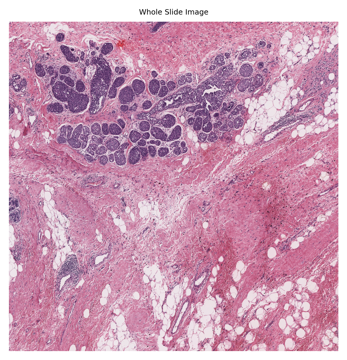
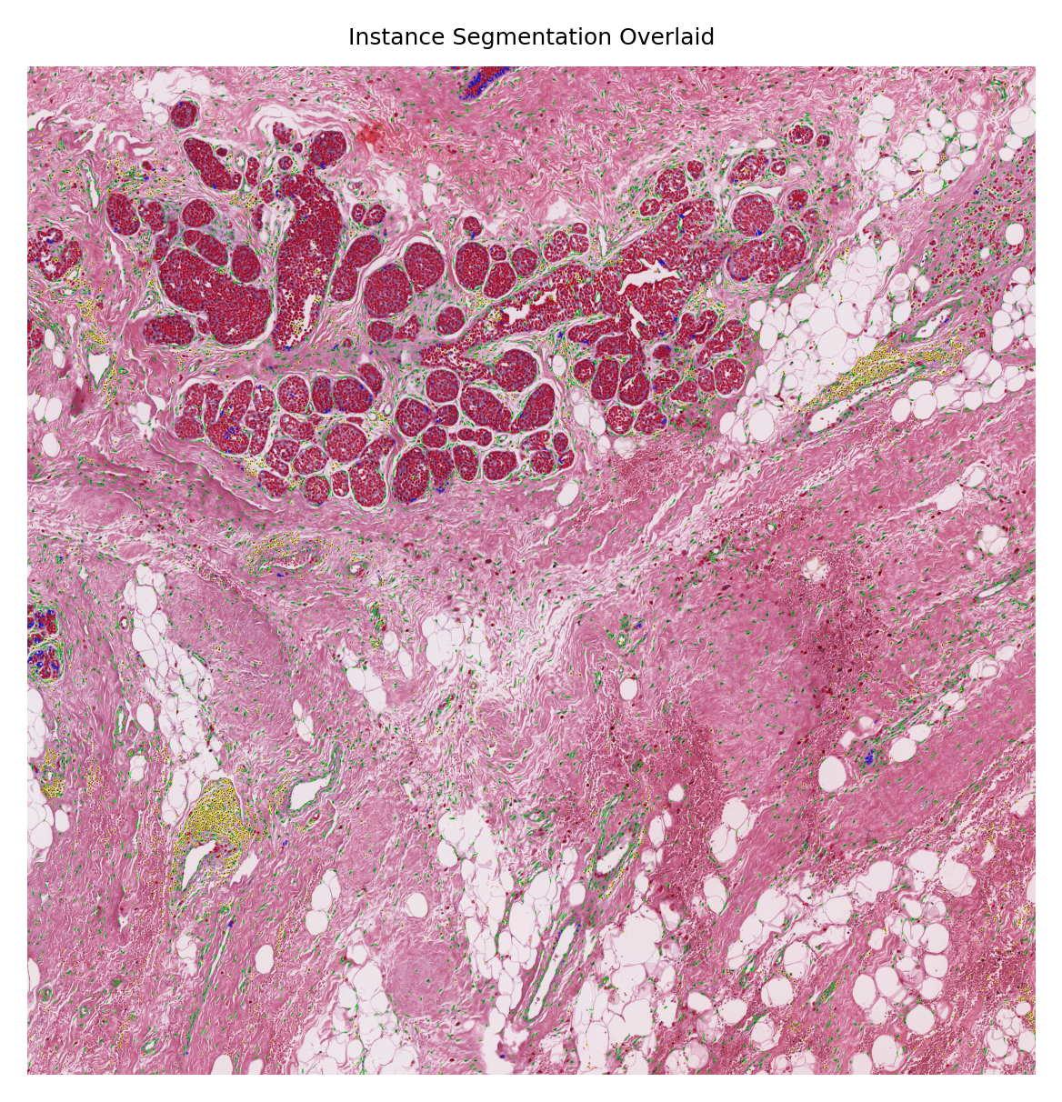
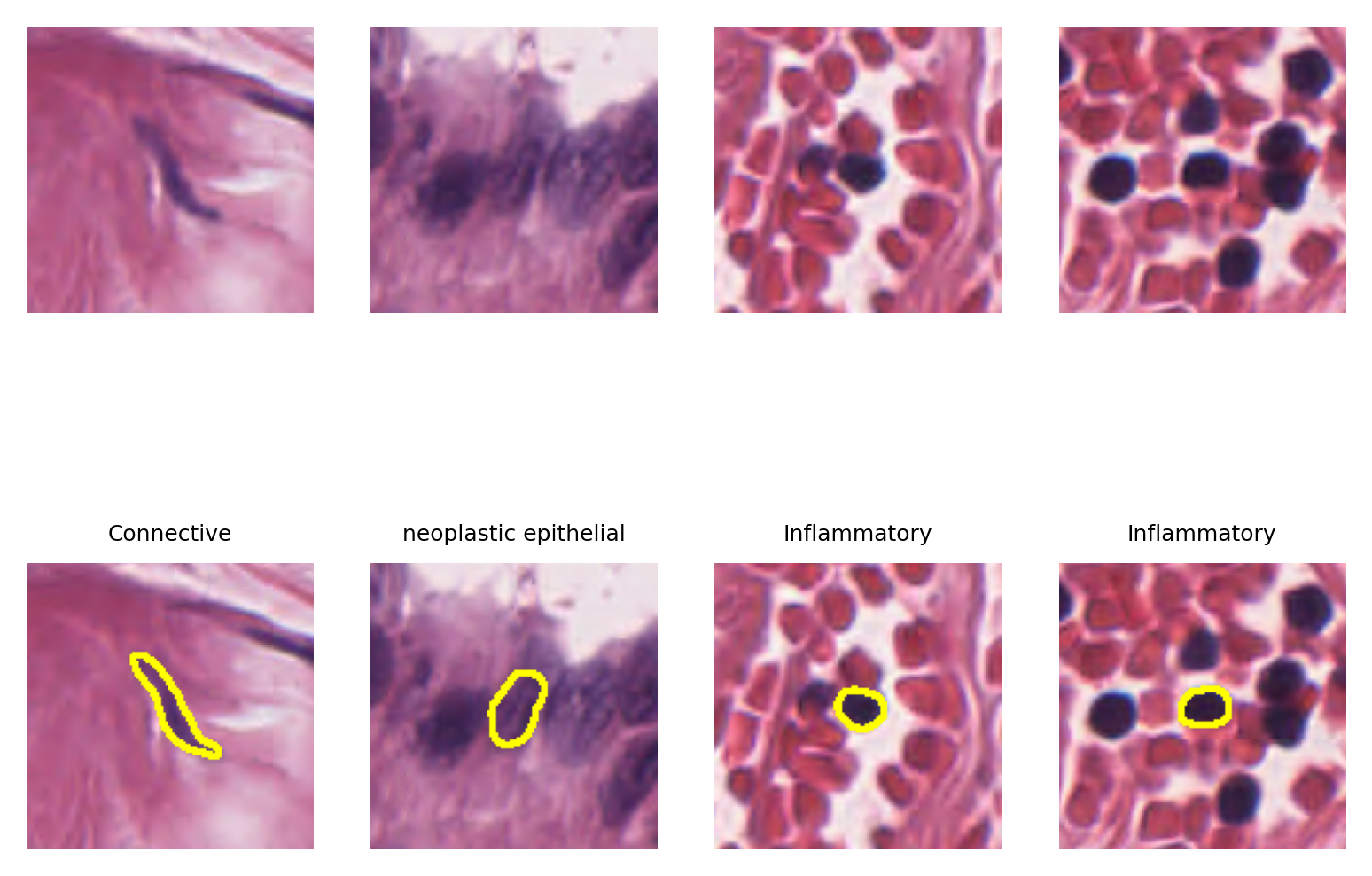
../../_images/eefd80adfe4a65a9620cb3a04f736fde6cafc8b42ef6d2abbba385e66a80e918.png

../../_images/467f71fcbeda9a263a7b8b308e348cf86ca24fdc48dc90af04e0aae42d338623.png

Although here we managed to overlay the results on the WSI (because this WSI is of size 12000x12000 which is relatively smaller than typical WSIs with pixels sizes larger than 100000x100000), we cannot distinguish a single nucleus in this big picture. However, to show the performance of the nucleus instance segmentation/classification, we will select four random nucleus instances and visualize them with their segmentation map overlaid on them. We will do this by leveraging the detected nucleus centroid information and read_rect functionality of the TIAToolbox WSI object.

bb = 128  # box size for patch extraction around each nucleus

for i in range(4):  # showing 4 examples
    selected_nuc_id = nuc_id_list[
        rng.integers(0, len(wsi_pred))
    ]  # randomly select a nucleus
    sample_nuc = wsi_pred[selected_nuc_id]
    cent = np.int32(
        sample_nuc["centroid"],
    )  # centroid position in WSI coordinate system
    contour = sample_nuc["contour"]  # nuceli contour points in WSI coordinate system
    contour -= (
        cent - bb // 2
    )  # nuceli contour points in the small patch coordinate system

    # Now reading the nucleus small window neighborhood
    nuc_patch = wsi.read_rect(
        cent - bb // 2,
        bb,
        resolution=0.25,
        units="mpp",
        coord_space="resolution",
    )
    # Overlay contour points on the extracted patch
    # using open-cv drawContours functionality
    overlaid_patch = cv2.drawContours(nuc_patch.copy(), [contour], -1, (255, 255, 0), 2)

    # plotting the results
    ax = plt.subplot(2, 4, i + 1), plt.imshow(nuc_patch), plt.axis("off")
    ax = (
        plt.subplot(2, 4, i + 5),
        plt.imshow(overlaid_patch),
        plt.axis("off"),
        plt.title(color_dict[sample_nuc["type"]][0]),
    )

../../_images/a0e8b22048d4274cfafd75894a7f4880c3df42da42931100cbfa61eb25b40c1b.png

How to visualize in TIAViz¶

TIAToolbox provides a flexible visualization tool for viewing slides and overlaying associated model outputs or annotations. It is a browser-based UI built using TIAToolbox and Bokeh. Below we show how to use this tool for our prediction example.

Note: To visualize the images and output on TIAViz, we recommend running the following code locally on your machine instead of Google Colab. Note: We have updated the output_type="annotationstore", which is the required output format to visualize the output of models in TIAViz.

# WSI prediction

class_dict = {
    "nuclei_segmentation": {
        0: "Background",
        1: "Neoplastic epithelial",
        2: "Inflammatory",
        3: "Connective",
        4: "Dead",
        5: "Non-neoplastic epithelial",
    }
}

wsi_output = inst_segmentor.run(
    images=[wsi_file_name],
    masks=None,
    patch_mode=False,
    save_dir=global_save_dir / "sample_wsi_results_annotationstore/",
    output_type="annotationstore",  # Set output type to annotationstore
    class_dict=class_dict,  # Provide class labels for annotation store
    auto_get_mask=False,
    num_workers=multiprocessing.cpu_count(),
)

Above, we run the NucleusInstanceSegmentor on WSI file wsi_file_name similar to the last time, but this time we specify a different value for the parameter output_type (output_type = "annotationstore"). In this case, the prediction results will be saved as .db files which are directly compatible with TIAViz.

Then, to start the TIAViz, simply use the command below, either in a terminal or by running the cell, and view localhost:5006 in your web browser.

%%bash
tiatoolbox visualize --slides ./tmp/ --overlays ./tmp/sample_wsi_results_annotationstore/

An example view you will have in your web browser is shown below. Make sure to click on Add Overlay button to select the corresponding overlay (sample_wsi.db) for your WSI (sample_wsi.svs). Try using different colors and changing options.

More details on visualization Interface usage can be found on [Visualization Interface Usage Documentation].

Example TIAViz Visualization:

In summary, it is very easy to use the pretrained HoVer-Net model in TIAToolbox to do nucleus instance segmentation and classification. You don’t even need to set any parameters related to a model’s input/output when you decide to work with one of TIAToolbox’s pretrained models (they will be set automatically, based on their optimal values). Here we explain how the parameters work, so we need to show them explicitly. In other words, nucleus instance segmentation in images/WSIs can be done as easily as:

segmentor = NucleusInstanceSegmentor(model="hovernet_fast-pannuke", num_workers=4, batch_size=4)
output = segmentor.run([img_file_name], patch_mode=True)

Feel free to play around with the parameters, models, and experiment with new images (just remember to run the first cell of this notebook again, so the created folders for the current examples would be removed or change the save_dir parameters in new calls of run function). If you want to use your pretrained model for instance segmentation (or any other pixel-wise prediction models) in the TIAToolbox framework, you can follow the instructions in our example notebook on