Semantic Segmentation Models
Click to open in: [GitHub][Colab]
About this demo
Semantic segmentation in image processing means partitioning the image into its constructing segments so that each segment corresponds to a specific category of an object present in the image. In other words, semantic segmentation can be considered as classifying each pixel in the image into a pre-defined category. Note that semantic segmentation does not differentiate instances of the same object, like the figure below which shows three examples of road images with their semantic segmentation. You can see how all objects of the same class have the same colour (please refer to here and here to find more information on the semantic segmentation task).
Image courtesy of: Chen, Liang-Chieh, et al. “Deeplab: Semantic image segmentation with deep convolutional nets, atrous convolution, and fully connected crfs.” IEEE transactions on pattern analysis and machine intelligence 40.4 (2017): 834-848.
Similar to natural images, semantic segmentation of histology images is the task of identifying the class of each pixel in the image based on the object or tissue type of the region encompassing that pixel. Semantic segmentation of tissue regions in histology images plays an important role in developing algorithms for cancer diagnosis and prognosis as it can help measure tissue attributes in an objective and reproducible fashion.
Example of semantic segmentation in histology images where pixels are classified based on different region types including tumour, fat, inflammatory, necrosis etc.
In this example notebook, we are showing how you can use pretrained models to do automatically segment different tissue region types in a set of input images or WSIs. We first focus on a pretrained model incorporated in the TIAToolbox to achieve semantic annotation of tissue region in histology images of breast cancer. After that, we will explain how you can use your pretrained model in the TIAToolbox model inference pipeline to do prediction on a set WSIs.
Downloading the required files
We download, over the internet, image files used for the purpose of this notebook. In particular, we download a histology tile and a whole slide image of cancerous breast tissue samples to show how semantic segmentation models work. Also, pretrained weights of a Pytorch model and a small WSI are downloaded to illustrate how you can incorporate your own models in the existing TIAToolbox segmentation tool.
In Colab, if you click the files icon (see below) in the vertical toolbar on the left hand side then you can see all the files which the code in this notebook can access. The data will appear here when it is downloaded.

data_dir = "./tmp"
if not Path(data_dir).exists():
    Path(data_dir).mkdir(exist_ok=True)


# Downloading sample image tile
img_file_name = hf_hub_download(
    repo_id="TIACentre/TIAToolBox_Remote_Samples",
    filename="sample_imgs/breast_tissue.jpg",
    repo_type="dataset",
    local_dir=data_dir,
)

# Downloading sample whole-slide image
wsi_file_name = hf_hub_download(
    repo_id="TIACentre/TIAToolBox_Remote_Samples",
    filename="sample_wsis/wsi4_12k_12k.svs",
    repo_type="dataset",
    local_dir=data_dir,
)

# Downloading mini whole-slide image
mini_wsi_file_name = hf_hub_download(
    repo_id="TIACentre/TIAToolBox_Remote_Samples",
    filename="sample_wsis/CMU-1.ndpi",
    repo_type="dataset",
    local_dir=data_dir,
)

# Download external model
model_file_name = hf_hub_download(
    repo_id="TIACentre/TIAToolbox_pretrained_weights",
    filename="fcn-tissue_mask.pth",
    repo_type="model",
    local_dir=data_dir,
)

logger.info("Download is complete.")
Semantic segmentation using TIAToolbox pretrained models
In this section, we will investigate the use of semantic segmentation models that have been already trained on a specific task and incorporated in the TIAToolbox. Particularly, the model we demonstrate can estimate the probability of each pixel in an image (tile or whole slide images) of breast cancer sample belonging to one of the following classes:
Tumour
Stroma
Inflammatory
Necrosis
Others (nerves, vessels, blood cells, adipose, etc.)
Inference on tiles
Much similar to the patch classifier functionality of the tiatoolbox, the semantic segmentation module works both on image tiles and structured WSIs. First, we need to create an instance of the SemanticSegmentor class which controls the whole process of semantic segmentation task and then use it to do prediction on the input image(s):
# Tile prediction
bcc_segmentor = SemanticSegmentor(
    model="fcn_resnet50_unet-bcss",
    num_workers=4,
    batch_size=4,
)

output = bcc_segmentor.run(
    images=[img_file_name],
    input_resolutions=[{"units": "baseline", "resolution": 1.0}],
    patch_input_shape=(1024, 1024),
    patch_output_shape=(512, 512),
    stride_shape=(512, 512),
    patch_mode=False,
    auto_get_mask=False,
    device=device,
    save_dir="./tmp/sample_tile_results/",
    return_probabilities=True,
)
There we go! With only two lines of code, thousands of WSIs can be processed automatically.
There are many parameters associated with SemanticSegmentor. We explain these as we meet them, while proceeding through the notebook. Here we explain only the ones mentioned above:
model: specifies the name of the pretrained model included in the TIAToolbox (case-sensitive). We are expanding our library of models pretrained on various segmentation tasks. You can find a complete list of available pretrained models here. In this example, we use the"fcn_resnet50_unet-bcss"pretrained model, which is a fully convolutional network that follows UNet network architecture and benefits from a ResNet50 model as its encoder part.num_workers: as the name suggests, this parameter controls the number of CPU cores (workers) that are responsible for the “loading of network input” process, which consists of patch extraction, preprocessing, and post-processing etc.batch_size: controls the batch size, or the number of input instances to the network in each iteration. If you use a GPU, be careful not to set thebatch_sizelarger than the GPU memory limit would allow.
After the bcc_segmentor has been instantiated as a semantic segmentation engine with our desired pretrained model, one can call the run method to do inference on a list of input images (or WSIs). The run function automatically processes all the images on the input list and saves the results on the disk. The process usually comprises patch extraction (because the whole tile or WSI won’t fit into limited GPU memory), preprocessing, model inference, post-processing and prediction assembly. There some important parameters that should be set to use the run method properly:
images: List of inputs to be processed. Note that items in the list should be paths to the inputs stored on the disk.input_resolutions: List of dictionaries with keys ‘units’ and ‘resolution’, specifying the resolution at which the input is processed. Because plain images only have a baseline layer, the options in this case should always be the defaultsunits="baseline"andresolution=1.0and, as defaults, can be omitted.patch_input_shape: the shape of the patches extracted from the input image (WSI) to be fed into the model. The bigger the patch size the more GPU memory is needed.patch_output_shape: The expected shape of output prediction maps for patches. This should be set based on the knowledge we have from the model design. For example, we know that the shape of output maps from"fcn_resnet50_unet-bcss"model is half of the input shape in each dimension. Therefore, as we set thepatch_input_shape=[1024, 1024]), we need to set thepatch_output_shape=[512, 512].stride_shape: Stride of output patches during tile and WSI processing. This parameter is used to set the amount of overlap between neighbouring prediction patches. Based on this parameter, the toolbox automatically calculates the patch extraction stride.patch_mode: Whether input is treated as patches (True) or WSIs (False). In this example, we process a tile image by dividing it into patches, sopatch_modeis set toFalse.auto_get_mask: Whether to automatically generate segmentation masks usingwsireader.tissue_mask()during processing.device: specify appropriate device e.g., “cuda”, “cuda:0”, “mps”, “cpu” etc.save_dir: Path to the main folder in which prediction results for each input will be stored separately.return_probabilities: Whether to return per-class probabilities.
We should mention that when you are using TIAToolbox pretrained models, you don’t need to worry about setting the input/output shape parameters as their optimal values will be loaded by default.
In the output, a list of the paths to its input files and the processed outputs saved on the disk is returned. This can be used for loading the results for processing and visualisation.
logger.info("Prediction method output is: %s", output)
logger.info(
"Key of the ouput is %s. Value of the output is %s",
Path(img_file_name),
output[Path(img_file_name)],
)
tile = imread(img_file_name)
logger.info(
"Input image dimensions: (%d, %d, %d)",
tile.shape[0],
tile.shape[1],
tile.shape[2],
)
zarr_prediction_raw = zarr.open(output[Path(img_file_name)], mode="r")
# Simple processing of the raw prediction to generate semantic segmentation task
tile_raw_prediction = da.from_zarr(zarr_prediction_raw["predictions"])
logger.info(
"Raw prediction dimensions: (%d, %d)",
tile_raw_prediction.shape[0],
tile_raw_prediction.shape[1],
)
tile_prediction = tile_raw_prediction[
: tile.shape[0], : tile.shape[1]
] # remove the extra borders to matches the input image size
logger.info(
"Processed prediction dimensions: (%d, %d)",
tile_prediction.shape[0],
tile_prediction.shape[1],
)
# Get probabilities of each class
tile_raw_probabilities = da.from_zarr(zarr_prediction_raw["probabilities"])
tile_probabilities_per_class = tile_raw_probabilities[
: tile.shape[0], : tile.shape[1], :
] # remove the extra borders to matches the input image size
logger.info(
"Processed probabilities dimensions: (%d, %d, %d)",
tile_probabilities_per_class.shape[0],
tile_probabilities_per_class.shape[1],
tile_probabilities_per_class.shape[2],
)
# showing the predicted semantic segmentation
fig = plt.figure()
label_names_dict = {
0: "Tumour",
1: "Stroma",
2: "Inflamatory",
3: "Necrosis",
4: "Others",
}
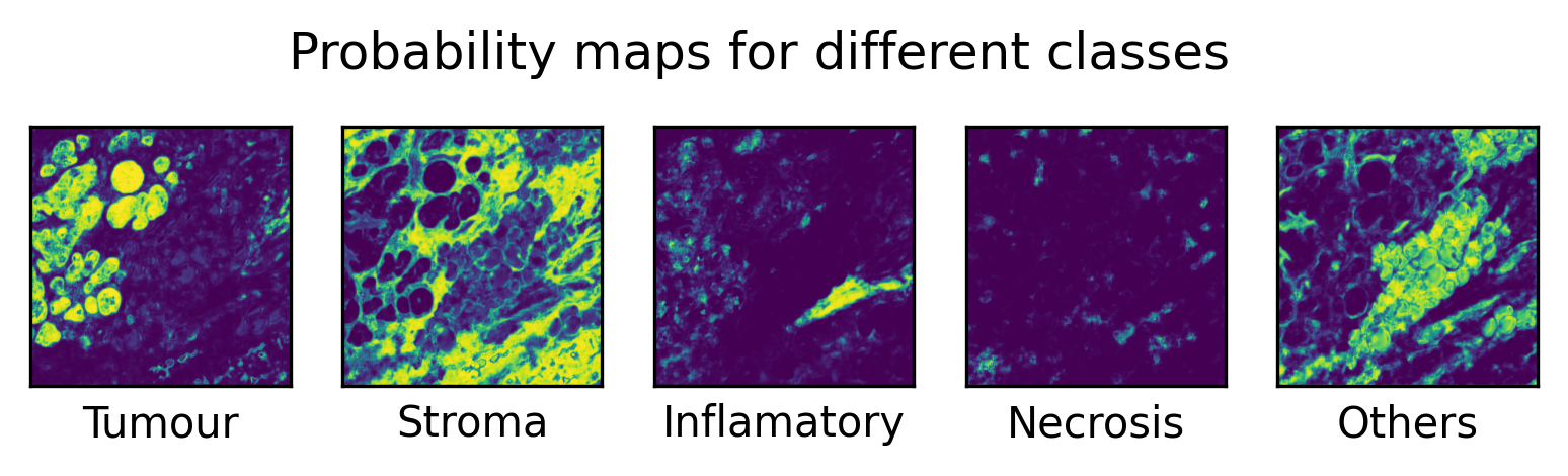
for i in range(5):
ax = plt.subplot(1, 5, i + 1)
(
plt.imshow(tile_probabilities_per_class[:, :, i]),
plt.xlabel(
label_names_dict[i],
),
ax.axes.xaxis.set_ticks([]),
ax.axes.yaxis.set_ticks([]),
)
fig.suptitle("Probability maps for different classes", y=0.65)
# showing processed results
fig2 = plt.figure()
ax1 = plt.subplot(1, 2, 1), plt.imshow(tile), plt.axis("off")
ax2 = plt.subplot(1, 2, 2), plt.imshow(tile_prediction), plt.axis("off")
fig2.suptitle("Processed prediction map", y=0.82)
|2026-02-02|12:09:34.451| [INFO] Prediction method output is: {PosixPath('tmp/sample_imgs/breast_tissue.jpg'): PosixPath('tmp/sample_tile_results/breast_tissue.zarr')}
|2026-02-02|12:09:34.452| [INFO] Key of the ouput is tmp/sample_imgs/breast_tissue.jpg. Value of the output is tmp/sample_tile_results/breast_tissue.zarr
|2026-02-02|12:09:34.772| [INFO] Input image dimensions: (4000, 4000, 3)
|2026-02-02|12:09:34.827| [INFO] Raw prediction dimensions: (4096, 4096)
|2026-02-02|12:09:34.828| [INFO] Processed prediction dimensions: (4000, 4000)
|2026-02-02|12:09:34.854| [INFO] Processed probabilities dimensions: (4000, 4000, 5)
Text(0.5, 0.82, 'Processed prediction map')
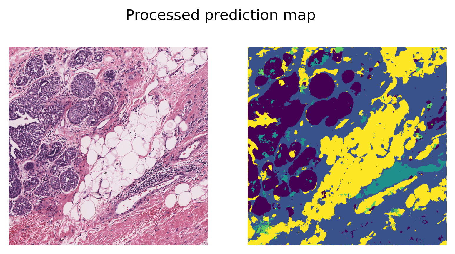
As printed above, when using the key predictions from the result dictionary, we obtain a single-channel prediction map, where each pixel value indicates the class label to which that pixel is assigned. A simple post-processing step is applied to remove the extra padded borders, ensuring that the prediction map matches the original input image size.
Alternatively, when using the key probabilities, the output is a five-channel probability map, where each channel corresponds to one tissue category. In this case, each pixel contains a probability value representing the likelihood of that pixel belonging to the corresponding tissue type. This multi-channel output provides a more detailed and interpretable representation of the model’s confidence across different tissue classes.
Inference on WSIs
The next step is to use the TIAToolbox’s embedded model for region segmentation in a whole slide image. The process is quite similar to what we have done for tiles. Here we just introduce a some important parameters that should be considered when configuring the segmentor for WSI inference.
bcc_segmentor = SemanticSegmentor(
    model="fcn_resnet50_unet-bcss",
    num_workers=4,
    batch_size=4,
)

bcc_wsi_ioconfig = IOSegmentorConfig(
    input_resolutions=[{"units": "mpp", "resolution": 0.25}],
    output_resolutions=[{"units": "mpp", "resolution": 0.25}],
    patch_input_shape=(1024, 1024),
    patch_output_shape=(512, 512),
    stride_shape=(512, 512),
)
When doing inference on WSIs, it is important to set the data stream configurations (such as input resolution, output resolution, size of merged predictions, etc.) appropriately for each model and application. In TIAToolbox, IOSegmentorConfig class is used to set these configurations as we have done in the above cell.
Parameters of IOSegmentorConfig have self-explanatory names, but let’s have look at their definition:
input_resolutions: a list specifying the resolution of each input head of model in the form of a dictionary. List elements must be in the same order as targetmodel.forward(). Of course, if your model accepts only one input, you just need to put one dictionary specifying'units'and'resolution'. But it’s good to know that TIAToolbox supports a model with more than one input!output_resolutions: a list specifying the resolution of each output head from model in the form of a dictionary. List elements must be in the same order as targetmodel.infer_batch().patch_input_shape: Shape of the largest input in (height, width) format.patch_output_shape: Shape of the largest output in (height, width) format.stride_shape: Stride in (y, x) direction for patch extraction.
# WSI prediction
wsi_output = bcc_segmentor.run(
    images=[wsi_file_name],
    masks=None,
    ioconfig=bcc_wsi_ioconfig,
    patch_mode=False,
    save_dir="./tmp/sample_wsi_results/",
    device=device,
    return_probabilities=True,
)
Note the only differences made here are:
masks=Nonein therunfunction:masksargument similar to theimagesshould be a list of paths to the desired image masks. Patches fromimagesare only processed if they are within a masked area of their correspondingmasks. If not provided (masks=None), then a tissue mask will be automatically generated for whole-slide images or the entire image is processed for image tiles.
The above cell might take a while to process, especially if you have set device="cpu". The processing time depends on the size of the input WSI and the selected resolution. Here, we have not specified any values, which means that the baseline resolution of the WSI, which is $40\times$ in this example, will be used.
logger.info("Prediction method output is: %s", wsi_output)
logger.info(
    "Key of the ouput is %s. Value of the output is %s",
    Path(wsi_file_name),
    wsi_output[Path(wsi_file_name)],
)

wsi = WSIReader.open(wsi_file_name)
logger.info(
    "WSI original dimensions: (%d, %d)",
    wsi.info.slide_dimensions[0],
    wsi.info.slide_dimensions[1],
)

zarr_prediction_raw = zarr.open(wsi_output[Path(wsi_file_name)], mode="r")
# Simple processing of the raw prediction to generate semantic segmentation task
wsi_raw_prediction = da.from_zarr(zarr_prediction_raw["predictions"])
logger.info(
    "Raw prediction dimensions: (%d, %d)",
    wsi_raw_prediction.shape[0],
    wsi_raw_prediction.shape[1],
)
wsi_prediction = wsi_raw_prediction[
    : wsi.info.slide_dimensions[0], : wsi.info.slide_dimensions[1]
]  # remove the extra borders to matches the input image size
logger.info(
    "Processed prediction dimensions: (%d, %d)",
    wsi_prediction.shape[0],
    wsi_prediction.shape[1],
)

# [WSI overview extraction]
# Now reading the WSI to extract it's overview
# extracting slide overview using `slide_thumbnail` method
overview_info = {"units": "mpp", "resolution": 2}
wsi_overview = wsi.slide_thumbnail(
    resolution=overview_info["resolution"],
    units=overview_info["units"],
)
logger.info(
    "WSI overview dimensions: (%d, %d)",
    wsi_overview.shape[0],
    wsi_overview.shape[1],
)
# produce overview of wsi semantic segmentation prediction
overview_resolution = overview_info["resolution"]
# Adjust the resolution of the predictions
prediction_resolution = bcc_wsi_ioconfig.output_resolutions[0]["resolution"]
scale_factor = (
    overview_resolution / prediction_resolution
)  # the scale factor between prediction and overview
wsi_prediction_overview = affine_transform(
    image=wsi_prediction,
    matrix=np.array([[scale_factor, 0.0], [0.0, scale_factor]]),
    output_shape=(wsi_overview.shape[0], wsi_overview.shape[1]),
)
plt.figure(), plt.imshow(wsi_overview)
plt.axis("off")

# [Overlay map creation]
# creating label-color dictionary to be fed into `overlay_prediction_mask` function
# to help generating color legend
label_dict = {"Tumour": 0, "Stroma": 1, "Inflamatory": 2, "Necrosis": 3, "Others": 4}
label_color_dict = {}
colors = cm.get_cmap("Set1").colors
for class_name, label in label_dict.items():
    label_color_dict[label] = (class_name, 255 * np.array(colors[label]))
# Creat overlay map using the `overlay_prediction_mask` helper function
overlay = overlay_prediction_mask(
    wsi_overview,
    np.array(wsi_prediction_overview),
    alpha=0.5,
    label_info=label_color_dict,
    return_ax=True,
)
|2026-02-02|12:15:33.967| [INFO] Prediction method output is: {PosixPath('tmp/sample_wsis/wsi4_12k_12k.svs'): PosixPath('tmp/sample_wsi_results/wsi4_12k_12k.zarr')}
|2026-02-02|12:15:33.968| [INFO] Key of the ouput is tmp/sample_wsis/wsi4_12k_12k.svs. Value of the output is tmp/sample_wsi_results/wsi4_12k_12k.zarr
|2026-02-02|12:15:34.413| [INFO] WSI original dimensions: (12000, 12000)
|2026-02-02|12:15:34.441| [INFO] Raw prediction dimensions: (12288, 12288)
|2026-02-02|12:15:34.443| [INFO] Processed prediction dimensions: (12000, 12000)
|2026-02-02|12:15:35.169| [INFO] WSI overview dimensions: (1503, 1503)
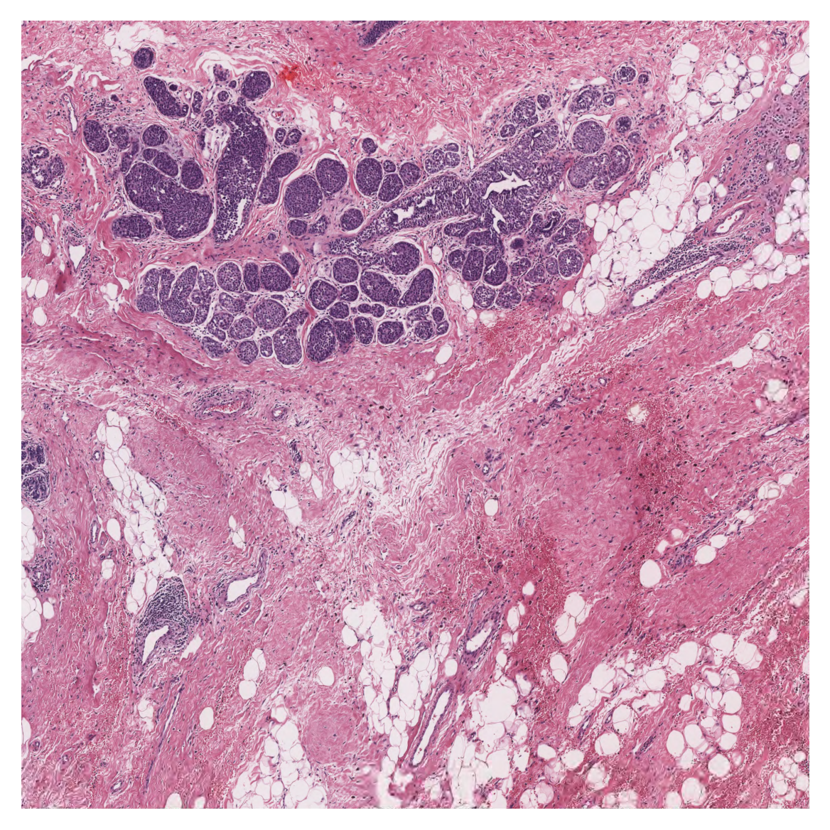
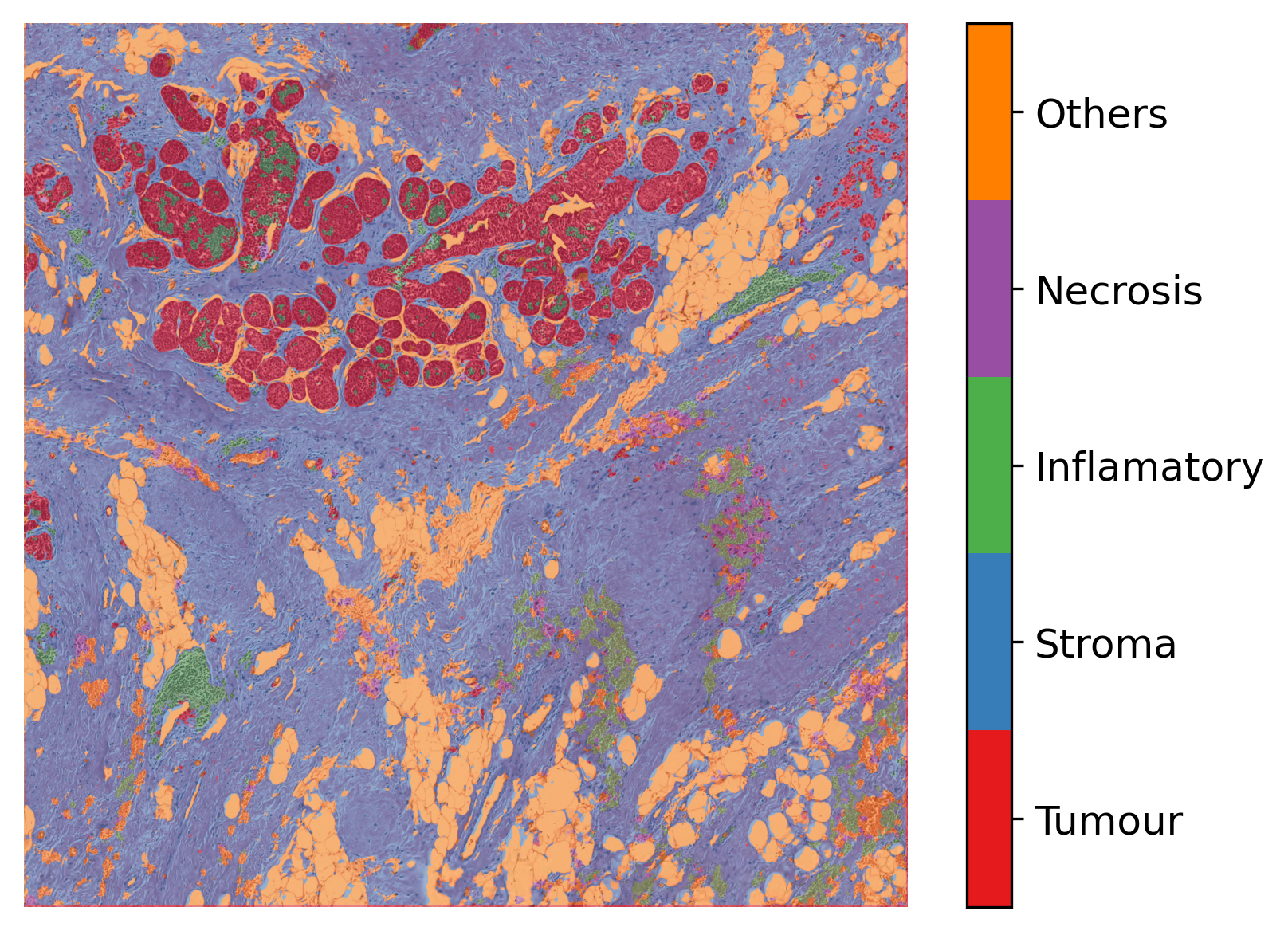
As you can see above, we first post-process the prediction map, the same way as we did for tiles, to create the semantic segmentation map. Then, in order to visualise the segmentation prediction on the tissue image, we read the processed WSI and extract its overview. We adjusted the resolution of prediction to match the WSI resolution. Finally, we used the overlay_prediction_mask helper function of the TIAToolbox to overlay the prediction map on the overview image and depict it with a colour legend.
In summary, it is very easy to use pretrained models in the TIAToolbox to do predefined tasks. In fact, you don’t even need to set any parameters related to a model’s input/output when you decide to work with one of TIAToolbox’s pretrained models (they will be set automatically, based on their optimal values). Here we explain how the parameters work, so we need to show them explicitly. In other words, region segmentation in images can be done as easily as:
segmentor = SemanticSegmentor(model="fcn_resnet50_unet-bcss", num_workers=4, batch_size=4)

output = segmentor.run(images=[img_file_name], input_resolutions=[{"units": "baseline", "resolution": 1.0}], patch_mode=False, auto_get_mask=False, save_dir="./tmp/sample_tile_results/")
In addition to the parameters shown in the previous examples, several other parameters can also be set for run method, as listed below.
overwrite: Whether to overwrite existing output files. Default isFalse.output_type: Desired output format: “dict”, “zarr”, or “annotationstore”. Default is"dict".class_dict: Mapping of classification outputs to class names.labels: Optional labels for input images. Only a single label per image is supported.memory_threshold: Memory usage threshold (percentage) to trigger caching behavior. This is recommended when processing large files. Try reducing the threshold if you get OOM errors consistently.output_file: Filename for saving output (e.g., “.zarr” or “.db”).return_labels: Whether to return labels with predictions.scale_factor: Scale factor for annotations (model_mpp / slide_mpp). Used to convert coordinates to baseline resolution.verbose: Whether to enable verbose logging.
Having said that, you may need to take care of a couple of other things if you want to use the same model with new weights, or even use a whole new model in the TIAToolbox inference pipeline. But don’t worry, these will be covered in the next section of this notebook.
Semantic segmentation using user-trained (external) models
At the TIACentre we are extending the number of pretrained models in the toolbox as fast as we can, to cover more tasks and tissue types. Nevertheless, users may need to use their own models in the TIAToolbox inference pipeline. In this case, TIAToolbox removes the burden of programing WSI processing, patch extraction, prediction aggregation, and multi-processing handling. Projects at scale provide further complications. But TIAToolbox comes to the rescue! TIAToolbox supports PyTorch models. It’s very easy to fit torch models in theTIAToolbox inference pipeline. We show you how.
Tissue segmentation model as an external model
We have a model that has been trained for tissue mask segmentation i.e., a PyTorch model that has been trained to distinguish between tissue and background, and we want to use it for tissue mask generation (instead of using a simple thresholding technique like Otsu’s method).
The first thing to do is to prepare our model. As an illustration of the technique, we use a generic UNet architecture that already been implemented in the TIAToolbox. The section “Downloading the required files” above describes downloading the weights pretrained for segmentation, and these are loaded into the model.
# define model architecture
external_model = UNetModel(
    num_input_channels=3,  # number of input image channels (3 for RGB)
    # number of model's output channels. 2 for two classes foreground and background.
    num_output_channels=2,
    # model used in the encoder part of the model to extract features
    encoder="resnet50",
    decoder_block=[
        3,
    ],  #  A list of convolution layers (each item specifies the kernel size)
)

# Loading pretrained weights into the model
map_location = torch.device(device)
pretrained_weights = torch.load(model_file_name, map_location=torch.device(device))
external_model.load_state_dict(pretrained_weights)
This is just an example, and you can use any CNN model of your choice. Remember that, in order to use SemanticSegmentor, model weights should already be loaded.
Now that we have our model in place, let’s create our SemanticSegmentor. Also, we need to configure the Input/Output stream of data for our model using IOSegmentorConfig.
tissue_segmentor = SemanticSegmentor(
    model=external_model,
    num_workers=4,
    batch_size=4,
)

# define the I/O configurations for tissue segmentation model
tissue_segmentor_ioconfig = IOSegmentorConfig(
    input_resolutions=[{"units": "mpp", "resolution": 2.0}],
    output_resolutions=[{"units": "mpp", "resolution": 2.0}],
    patch_input_shape=(1024, 1024),
    patch_output_shape=(512, 512),
    stride_shape=(512, 512),
)
Now, everything is in place to start the prediction using the defined tissue_segmentor on how many input images we like:
tissue_mask_output = tissue_segmentor.run(
    [mini_wsi_file_name],
    patch_mode=False,
    device=device,
    ioconfig=tissue_segmentor_ioconfig,
    save_dir="./tmp/tissue_mask_results/",
    return_probabilities=True,
)
If everything has gone well, tissue_segmentor should have been able to use our external model to do prediction on a whole slide image. Let’s see how well our model worked:
logger.info("Prediction method output is: %s", tissue_mask_output)
logger.info(
    "Key of the ouput is %s. Value of the output is %s",
    Path(mini_wsi_file_name),
    tissue_mask_output[Path(mini_wsi_file_name)],
)

# [WSI overview extraction]
# Now reading the WSI
mini_wsi = WSIReader.open(mini_wsi_file_name)
logger.info(
    "WSI original dimensions: (%d, %d)",
    mini_wsi.info.slide_dimensions[0],
    mini_wsi.info.slide_dimensions[1],
)
# Adjust the WSI resolution to match the input resolution
mini_wsi_input_info = {"units": "mpp", "resolution": 2.0}  # same as save_resolution
# extracting slide overview using `slide_thumbnail` method
mini_wsi_input = mini_wsi.slide_thumbnail(
    resolution=tissue_segmentor_ioconfig.input_resolutions[0]["resolution"],
    units=tissue_segmentor_ioconfig.input_resolutions[0]["units"],
)
logger.info(
    "WSI input dimensions: (%d, %d)",
    mini_wsi_input.shape[0],
    mini_wsi_input.shape[1],
)

# Loading the raw prediction
zarr_prediction_raw = zarr.open(tissue_mask_output[Path(mini_wsi_file_name)], mode="r")
mini_wsi_raw_prediction = da.from_zarr(zarr_prediction_raw["predictions"])
logger.info(
    "Raw prediction dimensions: (%d, %d)",
    mini_wsi_raw_prediction.shape[0],
    mini_wsi_raw_prediction.shape[1],
)
# Simple processing of the raw prediction to generate semantic segmentation task
mini_wsi_prediction = mini_wsi_raw_prediction[
    : mini_wsi_input.shape[0], : mini_wsi_input.shape[1]
]  # remove the extra borders to matches the input image size
logger.info(
    "Processed prediction dimensions: (%d, %d)",
    mini_wsi_prediction.shape[0],
    mini_wsi_prediction.shape[1],
)

# to create the wsi overview at a specific resolution
overview_info = {"units": "mpp", "resolution": 8.0}
# extracting slide overview using `slide_thumbnail` method
mini_wsi_overview = mini_wsi.slide_thumbnail(
    resolution=overview_info["resolution"],
    units=overview_info["units"],
)
logger.info(
    "WSI overview dimensions: (%d, %d)",
    mini_wsi_overview.shape[0],
    mini_wsi_overview.shape[1],
)

# Adjust the resolution of the predictions
overview_resolution = overview_info["resolution"]
prediction_resolution = tissue_segmentor_ioconfig.output_resolutions[0]["resolution"]
scale_factor = (
    overview_resolution / prediction_resolution
)  # the scale factor between prediction and overview resolution
mini_wsi_prediction_overview = affine_transform(
    image=mini_wsi_prediction,
    matrix=np.array([[scale_factor, 0.0], [0.0, scale_factor]]),
    output_shape=(mini_wsi_overview.shape[0], mini_wsi_overview.shape[1]),
)

ax = plt.subplot(1, 2, 1), plt.imshow(mini_wsi_overview)
plt.axis("off")
ax = plt.subplot(1, 2, 2), plt.imshow(mini_wsi_prediction)
plt.axis("off")
|2026-02-02|12:19:49.458| [INFO] Prediction method output is: {PosixPath('tmp/sample_wsis/CMU-1.ndpi'): PosixPath('tmp/tissue_mask_results/CMU-1.zarr')}
|2026-02-02|12:19:49.460| [INFO] Key of the ouput is tmp/sample_wsis/CMU-1.ndpi. Value of the output is tmp/tissue_mask_results/CMU-1.zarr
|2026-02-02|12:19:49.521| [INFO] WSI original dimensions: (51200, 38144)
|2026-02-02|12:20:41.257| [INFO] WSI input dimensions: (8679, 11684)
|2026-02-02|12:20:41.286| [INFO] Raw prediction dimensions: (8704, 11776)
|2026-02-02|12:20:41.288| [INFO] Processed prediction dimensions: (8679, 11684)
|2026-02-02|12:20:54.426| [INFO] WSI overview dimensions: (2170, 2921)
(np.float64(-0.5), np.float64(11683.5), np.float64(8678.5), np.float64(-0.5))
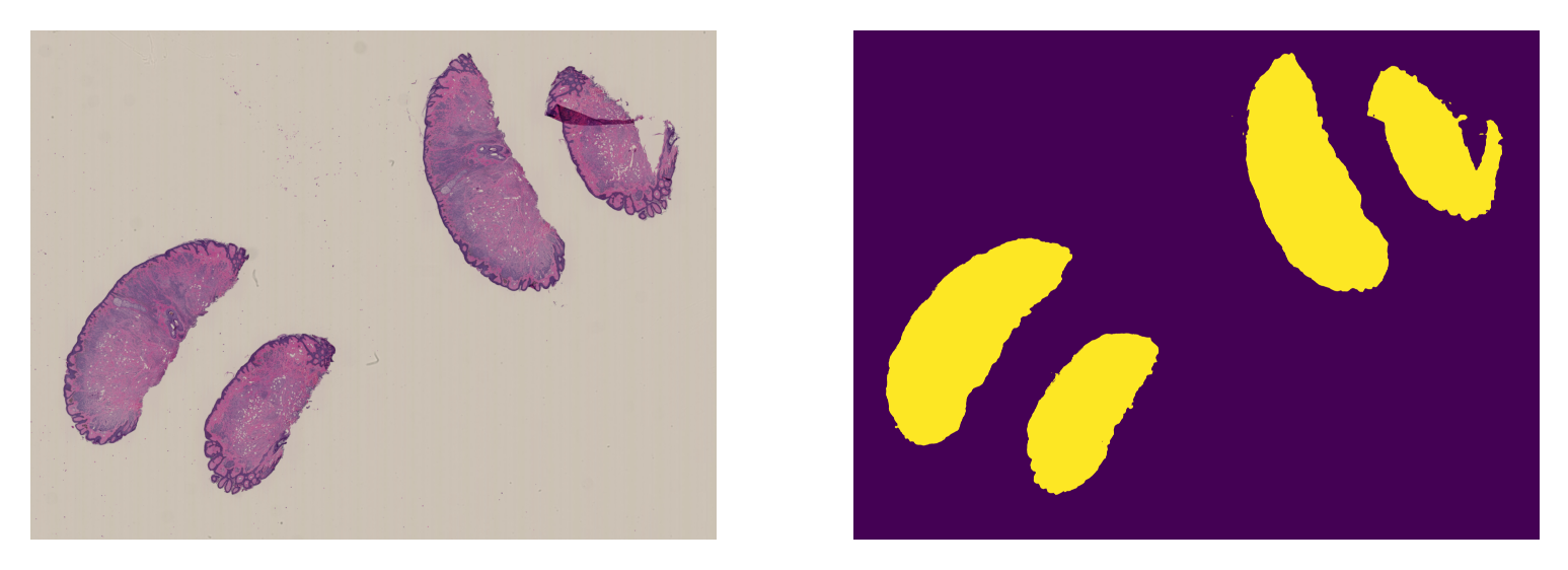
And that’s it!
To once again see how easy it is to use an external model in TIAToolbox’s semantic segmentation class, we summarize in pseudo-code, as below:
# 1- Define the Pytorch model and load weights
model = get_CNN()
model.load_state_dict(pretrained_weights)

# 2- Define the segmentor and IOconfig
segmentor = SemanticSegmentor(model)
ioconfig = IOSegmentorConfig(...)

# 3- Run the prediction
output = tissue_segmentor.run([img_paths], save_dir, ioconfig, ...)
Feel free to play around with the parameters, models, and experimenting with new images (just remember to run the first cell of this notebook again, so the created folders for the current examples would be removed or alternatively change the save_dir parameters in new calls of predict function). Currently, we are extending our collection of pre-trained models. To keep a track of them, make sure to follow our releases. You can also check here. Furthermore, if you want to use your own pretrained model for semantic segmentation (or any other pixel-wise prediction models) in the TIAToolbox framework, you can follow the instructions in our example notebook on advanced model techniques to gain some insights and guidance.
We welcome any trained model in computational pathology (in any task) for addition to TIAToolbox. If you have such a model (in Pytorch) and want to contribute, please contact us or simply create a PR on our GitHub page.
How to visualize in TIAViz
TIAToolbox provides a flexible visualization tool for viewing slides and overlaying associated model outputs or annotations. It is a browser-based UI built using TIAToolbox and Bokeh. Below we show how to use this tool for our prediction example.
Note that if you are running this notebook on Colab this step might not be for you.
wsi_output = bcc_segmentor.run(
    images=[wsi_file_name],
    masks=None,
    ioconfig=bcc_wsi_ioconfig,
    patch_mode=False,
    save_dir="./tmp/sample_wsi_results/",
    device=device,
    return_probabilities=True,
    output_type="annotationstore",
    overwrite=True,
    class_dict={0: "Tumour", 1: "Stroma", 2: "Inflamatory", 3: "Necrosis", 4: "Others"},
)
Above, we use SemanticSegmentor on WSI file wsi_file_name similar to the last time, but this time we specify a different value for the parameter output_type (output_type = "annotationstore"). In this case, the prediction results will be saved as .db files which are directly compatible with TIAViz.
Then, to start the TIAViz, simply use the command below, either in a terminal or by running the cell, and view localhost:5006 in your web browser.
%%bash
tiatoolbox visualize --slides ./tmp/sample_wsis/ --overlays ./tmp/sample_wsi_results/
An example view you will have in your web browser is shown below. Make sure to click on Add Overlay button to select the corresponding overlay (sample_wsi.db) for your WSI (sample_wsi.svs). Try using different colors and changing options.
More details on visualization Interface usage can be found on Visualization Interface Usage Documentation.
Example:

In this notebook, we show how we can use the SemanticSegmentor class and its run method to predict the semantic segmentation for tiles and WSIs. We show how to use overlay_prediction_mask helper function OR TIAViz to visualize the results as an overlay on the input image/WSI.
All the processes take place within TIAToolbox and you can easily put the pieces together, following our example code. Just make sure to set inputs and options correctly. We encourage you to further investigate the effect on the prediction output of changing run function parameters. Furthermore, if you want to use your own pretrained model for semantic segmentation in the TIAToolbox framework (even if the model structure is not defined in the TIAToolbox model class), you can follow the instructions in our example notebook on advanced model techniques to gain some insights and guidance.