Patch Prediction Models¶

Click to open in: [GitHub][Colab]

About this demo¶

In this example, we will show how to use TIAToolbox for patch-level prediction using a range of deep learning models. TIAToolbox can be used to make predictions on pre-extracted image patches or on larger image tiles / whole-slide images (WSIs), where image patches are extracted on the fly. WSI patch-level predictions can subsequently be aggregated to obtain a segmentation map. In particular, we will introduce the use of our module patch_predictor (details). A full list of the available models trained and provided in TIAToolbox for patch-level prediction is given below.

Models trained on the Kather 100k dataset (details):
- alexnet-kather100k
- resnet18-kather100k
- resnet34-kather100k
- resnet50-kather100k
- resnet101-kather100k
- resnext50_32x4d-kather100k
- resnext101_32x8d-kather100k
- wide_resnet50_2-kather100k
- wide_resnet101_2-kather100k
- densenet121-kather100k
- densenet161-kather100k
- densenet169-kather100k
- densenet201-kather100k
- mobilenet_v2-kather100k
- mobilenet_v3_large-kather100k
- mobilenet_v3_small-kather100k
- googlenet-kather100k

Downloading the required files¶

We download, over the internet, image files used for the purpose of this notebook. In particular, we download a sample subset of validation patches that were used when training models on the Kather 100k dataset, a sample image tile and a sample whole-slide image. Downloading is needed once in each Colab session and it should take less than 1 minute. In Colab, if you click the file’s icon (see below) in the vertical toolbar on the left-hand side then you can see all the files which the code in this notebook can access. The data will appear here when it is downloaded.

img_file_name = global_save_dir / "sample_tile.png"
wsi_file_name = global_save_dir / "sample_wsi.svs"
patches_file_name = global_save_dir / "kather100k-validation-sample.zip"
imagenet_samples_name = global_save_dir / "imagenet_samples.zip"

logger.info("Download has started. Please wait...")

# Downloading sample image tile
download_data(
    "https://tiatoolbox.dcs.warwick.ac.uk/sample_imgs/CRC-Prim-HE-05_APPLICATION.tif",
    img_file_name,
)

# Downloading sample whole-slide image
download_data(
    "https://tiatoolbox.dcs.warwick.ac.uk/sample_wsis/TCGA-3L-AA1B-01Z-00-DX1.8923A151-A690-40B7-9E5A-FCBEDFC2394F.svs",
    wsi_file_name,
)

# Download a sample of the validation set used to train the Kather 100K dataset
download_data(
    "https://tiatoolbox.dcs.warwick.ac.uk/datasets/kather100k-validation-sample.zip",
    patches_file_name,
)
# Unzip it!
with ZipFile(patches_file_name, "r") as zipfile:
    zipfile.extractall(path=global_save_dir)

# Download some samples of imagenet to test the external models
download_data(
    "https://tiatoolbox.dcs.warwick.ac.uk/sample_imgs/imagenet_samples.zip",
    imagenet_samples_name,
)
# Unzip it!
with ZipFile(imagenet_samples_name, "r") as zipfile:
    zipfile.extractall(path=global_save_dir)

logger.info("Download is complete.")

Get predictions for a set of patches¶

Below we use tiatoolbox to obtain the model predictions for a set of patches with a pretrained model.

We use patches from the validation subset of Kather 100k dataset. This dataset has already been downloaded in the download section above. We first read the data and convert it to a suitable format. In particular, we create a list of patches and a list of corresponding labels. For example, the first label in label_list will indicate the class of the first image patch in patch_list.

# read the patch data and create a list of patches and a list of corresponding labels

dataset_path = global_save_dir / "kather100k-validation-sample"

# set the path to the dataset
image_ext = ".tif"  # file extension of each image

# obtain the mapping between the label ID and the class name
label_dict = {
    "BACK": 0,
    "NORM": 1,
    "DEB": 2,
    "TUM": 3,
    "ADI": 4,
    "MUC": 5,
    "MUS": 6,
    "STR": 7,
    "LYM": 8,
}
class_names = list(label_dict.keys())
class_labels = list(label_dict.values())

# generate a list of patches and generate the label from the filename
patch_list = []
label_list = []
for class_name, label in label_dict.items():
    dataset_class_path = dataset_path / class_name
    patch_list_single_class = grab_files_from_dir(
        dataset_class_path,
        file_types="*" + image_ext,
    )
    patch_list.extend(patch_list_single_class)
    label_list.extend([label] * len(patch_list_single_class))


# show some dataset statistics
plt.bar(class_names, [label_list.count(label) for label in class_labels])
plt.xlabel("Patch types")
plt.ylabel("Number of patches")

# count the number of examples per class
for class_name, label in label_dict.items():
    logger.info(
        "Class ID: %d -- Class Name: %s -- Number of images: %d",
        label,
        class_name,
        label_list.count(label),
    )


# overall dataset statistics
logger.info("Total number of patches: %d", (len(patch_list)))

|2026-01-09|12:37:33.774| [INFO] Class ID: 0 -- Class Name: BACK -- Number of images: 211
|2026-01-09|12:37:33.775| [INFO] Class ID: 1 -- Class Name: NORM -- Number of images: 176
|2026-01-09|12:37:33.775| [INFO] Class ID: 2 -- Class Name: DEB -- Number of images: 230
|2026-01-09|12:37:33.776| [INFO] Class ID: 3 -- Class Name: TUM -- Number of images: 286
|2026-01-09|12:37:33.776| [INFO] Class ID: 4 -- Class Name: ADI -- Number of images: 208
|2026-01-09|12:37:33.777| [INFO] Class ID: 5 -- Class Name: MUC -- Number of images: 178
|2026-01-09|12:37:33.778| [INFO] Class ID: 6 -- Class Name: MUS -- Number of images: 270
|2026-01-09|12:37:33.778| [INFO] Class ID: 7 -- Class Name: STR -- Number of images: 209
|2026-01-09|12:37:33.779| [INFO] Class ID: 8 -- Class Name: LYM -- Number of images: 232
|2026-01-09|12:37:33.780| [INFO] Total number of patches: 2000

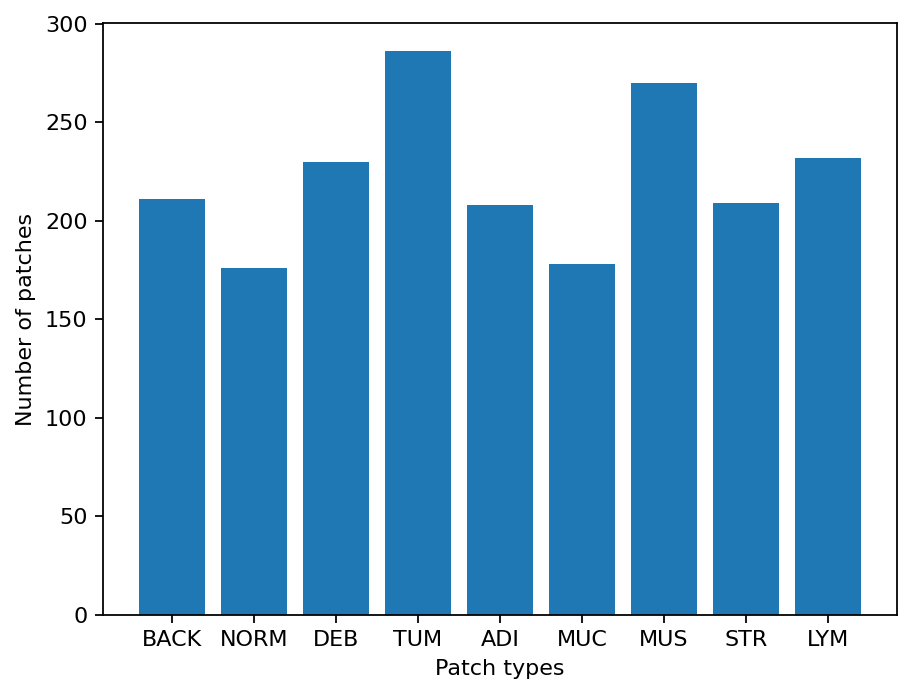
../../_images/5de87c983ee2e476d847b958bda90d6d0d2167e77d1ffb5658a3966b323f1393.png

As you can see for this patch dataset, we have 9 classes/labels with IDs 0-8 and associated class names. describing the dominant tissue type in the patch:

BACK ⟶ Background (empty glass region)
LYM ⟶ Lymphocytes
NORM ⟶ Normal colon mucosa
DEB ⟶ Debris
MUS ⟶ Smooth muscle
STR ⟶ Cancer-associated stroma
ADI ⟶ Adipose
MUC ⟶ Mucus
TUM ⟶ Colorectal adenocarcinoma epithelium

It is easy to use this code for your dataset - just ensure that your dataset is arranged like this example (images of different classes are placed into different subfolders), and set the right image extension in the image_ext variable.

Predict patch labels in 2 lines of code¶

Now that we have the list of images, we can use TIAToolbox’s PatchPredictor to predict their category. First, we instantiate a predictor object and then we call the run method to get the results.

predictor = PatchPredictor(model="resnet18-kather100k", batch_size=32)
output = predictor.run(
    patch_list,
    patch_mode=True,
    return_probabilities=True,
    device=device,
)

Patch Prediction is Done!

The first line creates a CNN-based patch classifier instance based on the arguments and prepares a CNN model (generates the network, downloads default weights, etc.). The model used in this predictor is specified with the model argument; to supply custom weights use the weights argument or pass a model instance. A complete list of supported pretrained classification models that have been trained on the Kather 100K dataset is reported in the first section of this notebook. PatchPredictor also enables you to use your own pretrained models for your specific classification application. In order to do that, you might need to change some input arguments for PatchPredictor, as we now explain:

model: You can pass the name of one of the pretrained models available in TIAToolbox, or pass a custom model instance. A list of pretrained models is available at the toolbox documentation. When passing a model name, default pretrained weights will be downloaded automatically (override via the weights argument). In this notebook we use resnet18-kather100k. You can use an externally defined PyTorch model for prediction, with weights already loaded. This is useful when you want to use your own pretrained model on your own data. The only constraint is that the input model should follow tiatoolbox.models.abc.ModelABC class structure. For more information on this matter, please refer to our example notebook on advanced model techniques.
weights: When providing a model name, the corresponding pretrained weights will be downloaded by default. You can override the default by passing a path to weights when constructing PatchPredictor.
batch_size: Number of images fed into the model each time. Higher values for this parameter require a larger (GPU) memory capacity.

The second line in the snippet above calls the run method to apply the CNN on the input patches and get the results. Here are some important run input arguments and their descriptions:

images: List of input images or patches. When using patch_mode=True, the input must be a list of images OR a list of image file paths, OR a Numpy array corresponding to an image list. However, when patch_mode=False, the images argument should be a list of paths to the input tiles or WSIs.
patch_mode: Whether to treat input as patches (True) or WSIs (False). Choose according to your application. In this first example, we predict the tissue type of histology patches, so we use the patch_mode=True option. patch_mode should be True if shape of input patches (height, width) is equal to the shape required by the input head of the model otherwise patch_mode should be False.
return_probabilities: set to True to get per class probabilities alongside predicted labels of input patches.

When patch_mode=True, the run method returns an output dictionary that contains the predictions (predicted labels) and probabilities (probability that a certain patch belongs to a certain class).

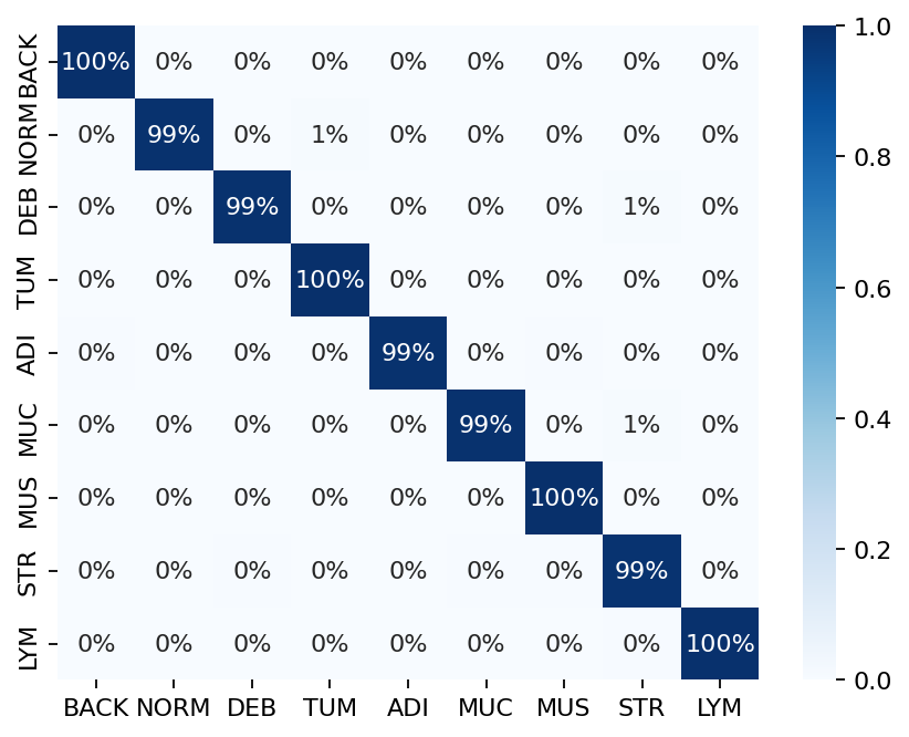
The cell below uses common python tools to visualize the patch classification results in terms of classification accuracy and confusion matrix.

acc = accuracy_score(label_list, output["predictions"])
logger.info("Classification accuracy: %f", acc)

# Creating and visualizing the confusion matrix for patch classification results
conf = confusion_matrix(label_list, output["predictions"], normalize="true")
df_cm = pd.DataFrame(conf, index=class_names, columns=class_names)

# show confusion matrix
sns.heatmap(df_cm, cmap="Blues", annot=True, fmt=".0%")
plt.show()

|2026-01-09|12:38:26.563| [INFO] Classification accuracy: 0.993000

../../_images/81c84e8b41cc01360280112e40252b7362cc3287bb6e39fa79e6d676b1ee75f6.png

Try changing the model argument when instantiating PatchPredictor and see how it can affect the classification output accuracy.

Get predictions for patches within an image tile¶

We now demonstrate how to obtain patch-level predictions for a large image tile. It is quite a common practice in computational pathology to divide a large image into several patches (often overlapping) and then aggregate the results to generate a prediction map for different regions of the large image. As we are making a prediction per patch again, there is no need to instantiate a new PatchPredictor class. However, we should tune the run input arguments to make them suitable for tile prediction. The run function then automatically extracts patches from the large image tile and predicts the label for each of them. The results will be saved in a specified location to avoid any problems with limited computer memory.

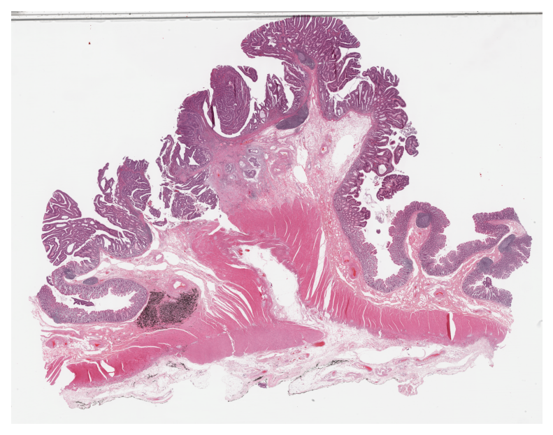
Now, we try this function on a sample image tile. For this example, we use a tile that was released with the Kather et al. 2016 paper. It has been already downloaded in the Download section of this notebook.

Let’s take a look.

# reading and displaying a tile image
input_tile = imread(img_file_name)

plt.imshow(input_tile)
plt.axis("off")
plt.show()

logger.info(
    "Tile size is: (%d, %d, %d)",
    input_tile.shape[0],
    input_tile.shape[1],
    input_tile.shape[2],
)

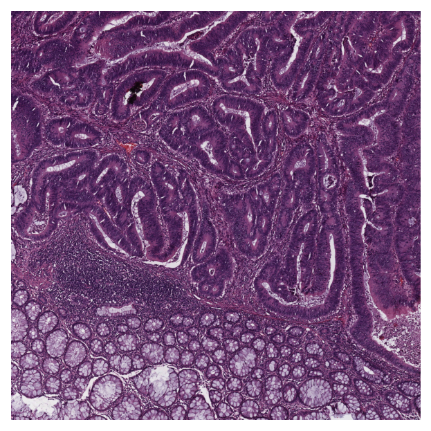
../../_images/96fd7e685f13afddf92210d0ba9916c5947e2cfa0c00410dcd936a335a50da8c.png

|2026-01-09|12:38:32.168| [INFO] Tile size is: (5000, 5000, 3)

Patch-level prediction in 2 lines of code for big histology tiles¶

As you can see, the size of the tile image is 5000x5000 pixels. This is quite big and might result in computer memory problems if fed directly into a deep learning model. However, the run method of PatchPredictor handles this big tile seamlessly by processing small patches independently. You only need to set patch_mode=False (and a couple of other arguments), as explained below.

rmdir(global_save_dir / "tile_predictions")
img_file_name = Path(img_file_name)

predictor = PatchPredictor(model="resnet18-kather100k", batch_size=32)
tile_output = predictor.run(
    images=[img_file_name],
    patch_mode=False,
    patch_input_shape=(224, 224),
    stride_shape=(224, 224),
    input_resolutions=[{"units": "baseline", "resolution": 1.0}],
    return_probabilities=True,
    auto_get_mask=False,
    save_dir=global_save_dir / "tile_predictions",
    device=device,
)

|2026-01-09|12:38:35.820| [WARNING] GPU is not compatible with torch.compile. Compatible GPUs include NVIDIA V100, A100, and H100. Speedup numbers may be lower than expected.

|2026-01-09|12:38:35.822| [INFO] output_type has been updated to 'zarr' for saving the file to tmp/tile_predictions.Remove `save_dir` input to return the output as a `dict`.
|2026-01-09|12:38:36.014| [INFO] When providing multiple whole slide images, the outputs will be saved and the locations of outputs will be returned to the calling function when `run()` finishes successfully.

|2026-01-09|12:38:36.961| [WARNING] Raw data is None.
|2026-01-09|12:38:36.962| [WARNING] Unknown scale (no objective_power or mpp)

|2026-01-09|12:38:38.950| [INFO] Saving output to tmp/tile_predictions/sample_tile.zarr.
[########################################] | 100% Completed | 103.20 ms
|2026-01-09|12:38:39.080| [INFO] Output file saved at tmp/tile_predictions/sample_tile.zarr.

The new arguments in the input of run method are:

patch_mode=False: the type of image input (tile mode for large images).
images: in tile mode, the input is required to be a list of file paths.
save_dir: directory to save output files. Required for tile/WSI mode. For each tile a .zarr file is written to save_dir.
patch_input_shape: size of patches (in [H, W]) that will be extracted from each tile.
stride_shape: stride (in [H, W]) between consecutive patches. A smaller stride produces overlapping patches.
input_resolutions: controls the scale at which tiles are read. Setting it to [{'units': 'baseline', 'resolution': 1.0}].
auto_get_mask=False: disables automatic tissue mask generation.

Load the output tile predictions from disk¶

The returned dictionary tile_output maps each tile path to its corresponding .zarr file. We load the output tile predictions into memory as below.

tile_output

{PosixPath('tmp/sample_tile.png'): PosixPath('tmp/tile_predictions/sample_tile.zarr')}

tile_output is a Python dictionary. To access output corresponding to a particular image, you can use the image file name img_file_name as a key to the tile_output dictionary as below.

store_path = tile_output[img_file_name]
tile_predictions = zarr.open(store_path, mode="r")
logger.info(f"Output keys: {list(tile_predictions.keys())}")

|2026-01-09|12:40:10.101| [INFO] Output keys: ['coordinates', 'predictions', 'probabilities']

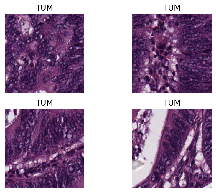
Visualisation of tile results¶

Below we show some of the results generated by our patch-level predictor on the input image tile. First, we will show some individual patch predictions and then we will show the merged patch level results on the entire image tile.

# individual patch predictions sampled from the image tile

coordinates = tile_predictions["coordinates"]
predictions = tile_predictions["predictions"]

# select 4 random indices (patches)
rng = np.random.default_rng()  # Numpy Random Generator
random_idx = rng.integers(0, len(predictions), (4,))

for i, idx in enumerate(random_idx):
    this_coord = coordinates[idx]
    this_prediction = predictions[idx]
    this_class = class_names[this_prediction]

    this_patch = input_tile[
        this_coord[1] : this_coord[3],
        this_coord[0] : this_coord[2],
    ]
    plt.subplot(2, 2, i + 1), plt.imshow(this_patch)
    plt.axis("off")
    plt.title(this_class)

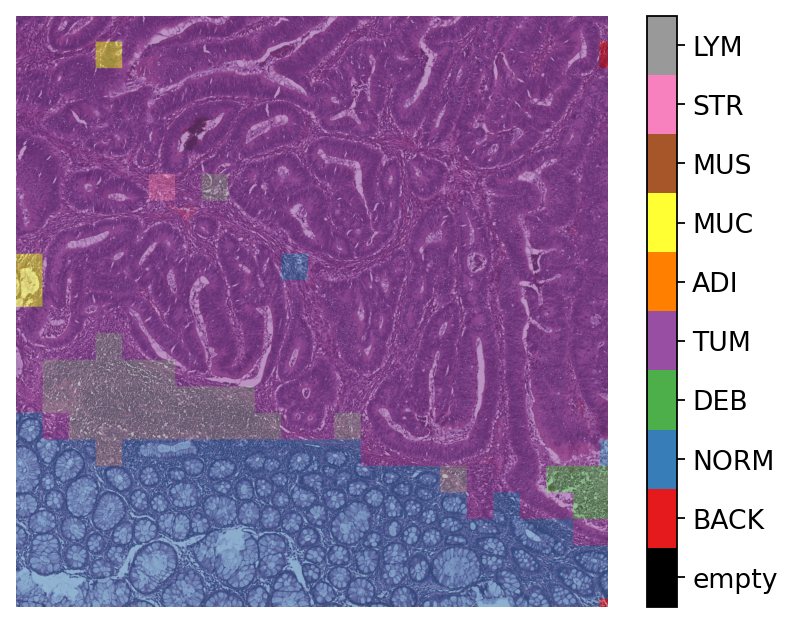
../../_images/b8e07b4bd3b366ae00cc84be470923e0f8c7afd8738cc4fc8404b8ca2a5d0c73.png

Here, we generate and show a prediction map in which regions have indexed values based on their classes. We overlay this prediction map on the original image, where each colour denotes a different predicted category. To generate this prediction map, we utilize the predictor outputs tile_predictions["predictions"] and tile_predictions["coordinates"] as below.

# simple merge patch predictions to generate tile-level prediction map

H, W = input_tile.shape[:2]
preds = np.asarray(tile_predictions["predictions"])
coords = np.asarray(tile_predictions["coordinates"])

pred_map = np.zeros((H, W), dtype=np.uint8)
for p, (x1, y1, x2, y2) in zip(preds, coords, strict=False):
    pred_map[int(y1) : int(y2), int(x1) : int(x2)] = int(p) + 1

To visualize the prediction map as an overlay on the input image, we use the overlay_prediction_mask function from the tiatoolbox.utils.visualization module. It accepts as arguments the original image, the prediction map, the alpha parameter which specifies the blending ratio of overlay and original image, and the label_info dictionary which contains names and desired colours for different classes. Below we generate an example of an acceptable label_info dictionary and show how it can be used with overlay_patch_prediction.

# visualization of merged image tile patch-level prediction

label_color_dict = {}
label_color_dict[0] = ("empty", (0, 0, 0))
colors = cm.get_cmap("Set1").colors
for class_name, label in label_dict.items():
    label_color_dict[label + 1] = (class_name, 255 * np.array(colors[label]))

overlay = overlay_prediction_mask(
    input_tile,
    pred_map,
    alpha=0.5,
    label_info=label_color_dict,
    return_ax=True,
)
plt.show()

../../_images/e015e273e02ef67d24e0b3574ba474861c087b94adc348f76fcbc3b039fbb471.png

Note that overlay_prediction_mask returns a figure handler, so that plt.show() or plt.savefig() shows or, respectively, saves the overlay figure generated. Now go back and predict with a different pretrained_model to see what effect this has on the output.

Get predictions for patches within a WSI¶

We demonstrate how to obtain predictions for all patches within a whole slide image. As in previous sections, we will use PatchPredictor and its run method, and set patch_mode=False. We also introduce IOPatchPredictorConfig, a class that specifies the configuration of image reading and prediction writing for the model prediction engine.

wsi_ioconfig = IOPatchPredictorConfig(
    input_resolutions=[{"units": "mpp", "resolution": 0.5}],
    patch_input_shape=[224, 224],
    stride_shape=[224, 224],
)

Parameters of IOPatchPredictorConfig have self-explanatory names, but let’s have look at their definition:

input_resolutions: a list specifying the resolution of each input head of model in the form of a dictionary. List elements must be in the same order as target model.forward(). Of course, if your model accepts only one input, you just need to put one dictionary specifying 'units' and 'resolution'. But it’s good to know that TIAToolbox supports a model with more than one input.
patch_input_shape: Shape of the largest input in (height, width) format.
stride_shape: the size of stride (steps) between two consecutive patches, used in the patch extraction process. If the user sets stride_shape equal to patch_input_shape, patches will be extracted and processed without any overlap.

Now that we have set everything, we try our patch predictor on a WSI. Here, we use a large WSI and therefore the patch extraction and prediction processes may take some time (make sure to set the device="cuda" if you have access to cuda enabled GPU).

predictor = PatchPredictor(model="resnet18-kather100k", batch_size=64)
wsi_output = predictor.run(
    images=[wsi_file_name],
    masks=None,
    patch_mode=False,
    ioconfig=wsi_ioconfig,
    return_probabilities=True,
    save_dir=global_save_dir / "wsi_predictions",
    device=device,
)

We introduce some new arguments for run method:

ioconfig: set the IO configuration information using the IOPatchPredictorConfig class.
masks: expects a list of paths to specify the regions in the original WSIs from which we want to extract patches. If None and the auto_get_mask is not False (default value is True), tissue masks will be generated automatically as in our example.

Then, we load the output into memory:

# Load the output
store_path = wsi_output[wsi_file_name]
wsi_predictions = zarr.open(store_path, mode="r")

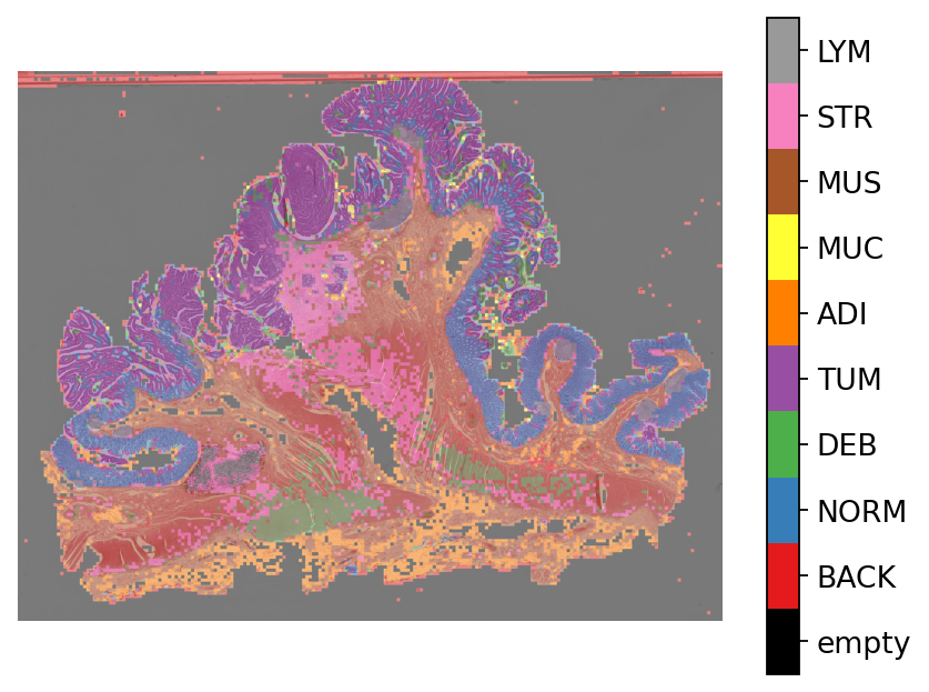
Finally, similar to how we visualized the tile results, we generate and visualize the prediction map as an overlay on the input WSI below.

Here, note the usage of a new scale_factor to scale between prediction and overview resolutions.

# visualization of whole slide image patch prediction

overview_resolution = (
    4  # the resolution in which we desire to merge and visualize the patch predictions
)

prediction_resolution = 0.5  # the resolution at which the patch predictions were made

# the unit of the `resolution` parameter. Can be "power", "level", "mpp", or "baseline"
unit = "mpp"

# get WSI overview image
wsi = WSIReader.open(wsi_file_name)
wsi_overview = wsi.slide_thumbnail(resolution=overview_resolution, units=unit)
plt.figure(), plt.imshow(wsi_overview)
plt.axis("off")


# Merge patch predictions to generate a 2D prediction map
H, W = wsi_overview.shape[:2]
preds = np.asarray(wsi_predictions["predictions"])
coords = np.asarray(wsi_predictions["coordinates"])

scale_factor = (
    overview_resolution / prediction_resolution
)  # the scale factor between prediction and overview resolution

pred_map = np.zeros((H, W), dtype=np.uint8)
for p, (x1, y1, x2, y2) in zip(preds, coords, strict=False):
    x1_ = x1 / scale_factor
    x2_ = x2 / scale_factor
    y1_ = y1 / scale_factor
    y2_ = y2 / scale_factor
    pred_map[int(y1_) : int(y2_), int(x1_) : int(x2_)] = int(p) + 1

../../_images/cd82bdb30e2b1b3a64ba00ed06c24728dc9e93dab5a5948df27280df76a90dd1.png

# Plotting the prediction map on WSI overview
overlay = overlay_prediction_mask(
    wsi_overview,
    pred_map,
    alpha=0.5,
    label_info=label_color_dict,
    return_ax=True,
)
plt.show()

../../_images/28fcb4f244abce46d07e81d17dd8858e58229d9709d2107726a9d6be963cb6e8.png

How to visualize in TIAViz¶

TIAToolbox provides a flexible visualization tool for viewing slides and overlaying associated model outputs or annotations. It is a browser-based UI built using TIAToolbox and Bokeh. Below we show how to use this tool for our prediction example.

Note: To visualize the images and output on TIAViz, we recommend running the following code locally on your machine instead of Google Colab.

predictor = PatchPredictor(model="resnet18-kather100k", batch_size=64)
class_dict = {v: k for k, v in label_dict.items()}

wsi_output = predictor.run(
    images=[wsi_file_name],
    masks=None,
    patch_mode=False,
    ioconfig=wsi_ioconfig,
    return_probabilities=True,
    save_dir=global_save_dir / "wsi_predictions_annotationstore",
    device=device,
    class_dict=class_dict,  # Provide class labels for annotation store
    output_type="annotationstore",  # Set output type to annotationstore
)
wsi_output

Above, we use PatchPredictor on WSI file wsi_file_name similar to the last time, but this time we specify a different value for the parameter output_type (output_type = "annotationstore"). In this case, the prediction results will be saved as .db files which are directly compatible with TIAViz.

Then, to start the TIAViz, simply use the command below, either in a terminal or by running the cell, and view localhost:5006 in your web browser.

%%bash
tiatoolbox visualize --slides ./tmp/ --overlays ./tmp/wsi_predictions_annotationstore/

An example view you will have in your web browser is shown below. Make sure to click on Add Overlay button to select the corresponding overlay (sample_wsi.db) for your WSI (sample_wsi.svs). Try using different colors and changing options.

More details on visualization Interface usage can be found on [Visualization Interface Usage Documentation].

Example TIAViz Visualization:

In this notebook, we show how we can use the PatchPredictor class and its run method to predict the label for patches of big tiles and WSIs. We show how to use overlay_prediction_mask helper function OR TIAViz to visualize the results as an overlay on the input image/WSI.

All the processes take place within TIAToolbox and you can easily put the pieces together, following our example code. Just make sure to set inputs and options correctly. We encourage you to further investigate the effect on the prediction output of changing run function parameters. Furthermore, if you want to use your own pretrained model for patch classification in the TIAToolbox framework (even if the model structure is not defined in the TIAToolbox model class), you can follow the instructions in our example notebook on advanced model techniques to gain some insights and guidance.